After cancer is diagnosed, healthcare providers need to learn as much as they can about it. This helps them to plan the best treatment and look at overall outcomes and goals. For many types of cancer, part of this process includes figuring out the cancer grade and stage. Bsed on patient’s medical history, our data-driven models can predict the cancer grades thus acting as a deicision suport tool for the healthcare providers.

Background

What is Colon cancer?

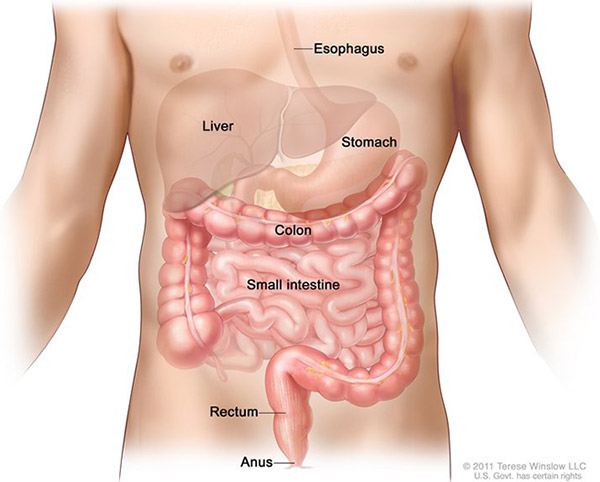
Cancer that begins in the colon is called colon cancer, and cancer that begins in the rectum is called rectal cancer. Cancer that starts in either of these organs may also be called colorectal cancer. The digestive system is made up of the esophagus, stomach, and the small and large intestines. The first 6 feet of the large intestine are called the large bowel or colon. The last 6 inches are the rectum and the anal canal.

Colorectal cancer is the fourth most common cancer diagnosed in the United States.Based on 2014-2016 data, approximately 4.2 percent of men and women will be diagnosed with colorectal cancer at some point during their lifetime.

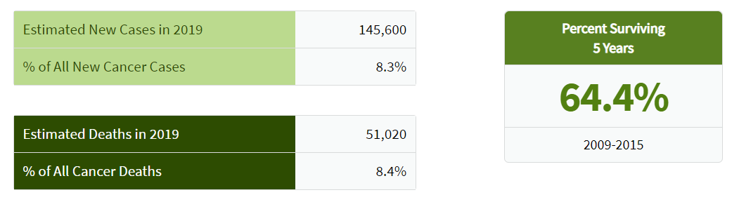
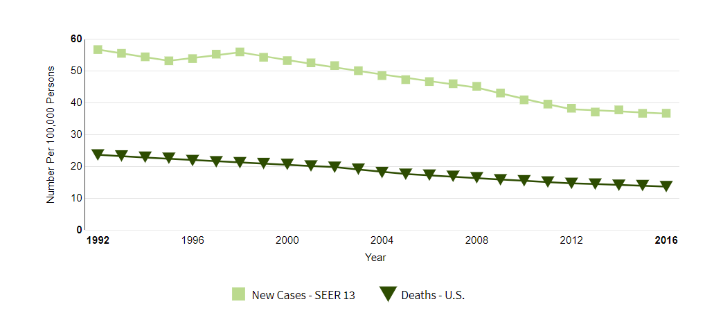
The number of new cases of colorectal cancer was 38.6 per 100,000 men and women per year. The number of deaths was 14.2 per 100,000 men and women per year. These rates are age-adjusted and based on 2012-2016 cases and deaths.

In 2016, there were an estimated 1,324,922 people living with colorectal cancer in the United States.

Cancer Grades

The grade of a cancer depends on what the cells look like under a microscope.

In general, a lower grade indicates a slower-growing cancer and a higher grade indicates a faster-growing one. The grading system that’s usually used is as follows:

grade I – cancer cells that resemble normal cells and aren’t growing rapidly
grade II – cancer cells that don’t look like normal cells and are growing faster than normal cells
grade III – cancer cells that look abnormal and may grow or spread more aggressively

Source of Data

The data is obtained from the Surveillance, Epidemiology, and End Results (SEER) Program. SEER provides information on cancer statistics in an effort to reduce the cancer burden among the U.S. population. SEER is supported by the Surveillance Research Program (SRP) in NCI’s Division of Cancer Control and Population Sciences (DCCPS).

https://seer.cancer.gov/data/access.html

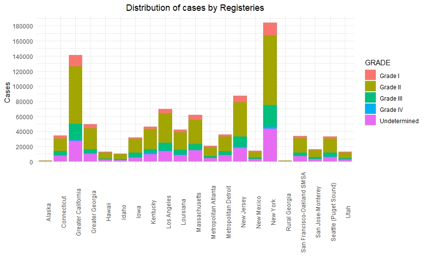
The Surveillance, Epidemiology, and End Results (SEER) Program of the National Cancer Institute (NCI) collects and publishes cancer data through a coordinated system of strategically placed cancer registries which cover near 30% of the USA population. Currently there are 18 SEER registries in the USA.

The 2000-2016 colon/rectal cancer dataset has 939,119 records, 35 columns and has a file size of 200 MB.

Data Analysis and Modeling

Pre-processing

Data preprocessing was a major part of this project. The data was made available in ASCII file format. So we first had convert it into CSV with a snipped of code in python.

Once we were able to parse these ASCII files, the next task was to decode the information in the data. Most of the attributes were represented with medical codes and had to be decoded according to the data dictionary.

After decoding, it was noticed that a lot of attributes possessed high cardinality. It was impossible to deal with that without medical expertise of the field. We tried a simplistic approach first in this regard and grouped together the minority classes.

Once this was done, the next task was to encode the data again to make it compatible with Python’s sci-kit library. We had to encode it carefully as some attributes required one hot encoding whereas label encoding was enough for some.

After encoding, our number of attributes increased tenfold, and naturally then feature engineering was the next step.

Feature Engineering

Feature engineering is an important step whenever you are working with data with extraordinarily large number of attributes. It helps in both – eliminating the redundancies in the data as well as saving the computational effort.

To reduce the number of attributes, we ran first a pairwise correlation test, which showed us that more than 25% of the attributes were redundant. The threshold selected here was 90%; i.e. the features with 90% or more correlation were eliminated.

PCA is also a good approach but was not used in this case since, our numerical data came from encoding and not actual measurements.

The third strategy we implemented was – Permutation Importance and Partial Dependence. These two are unique ways to calculate practical importance of each attribute.

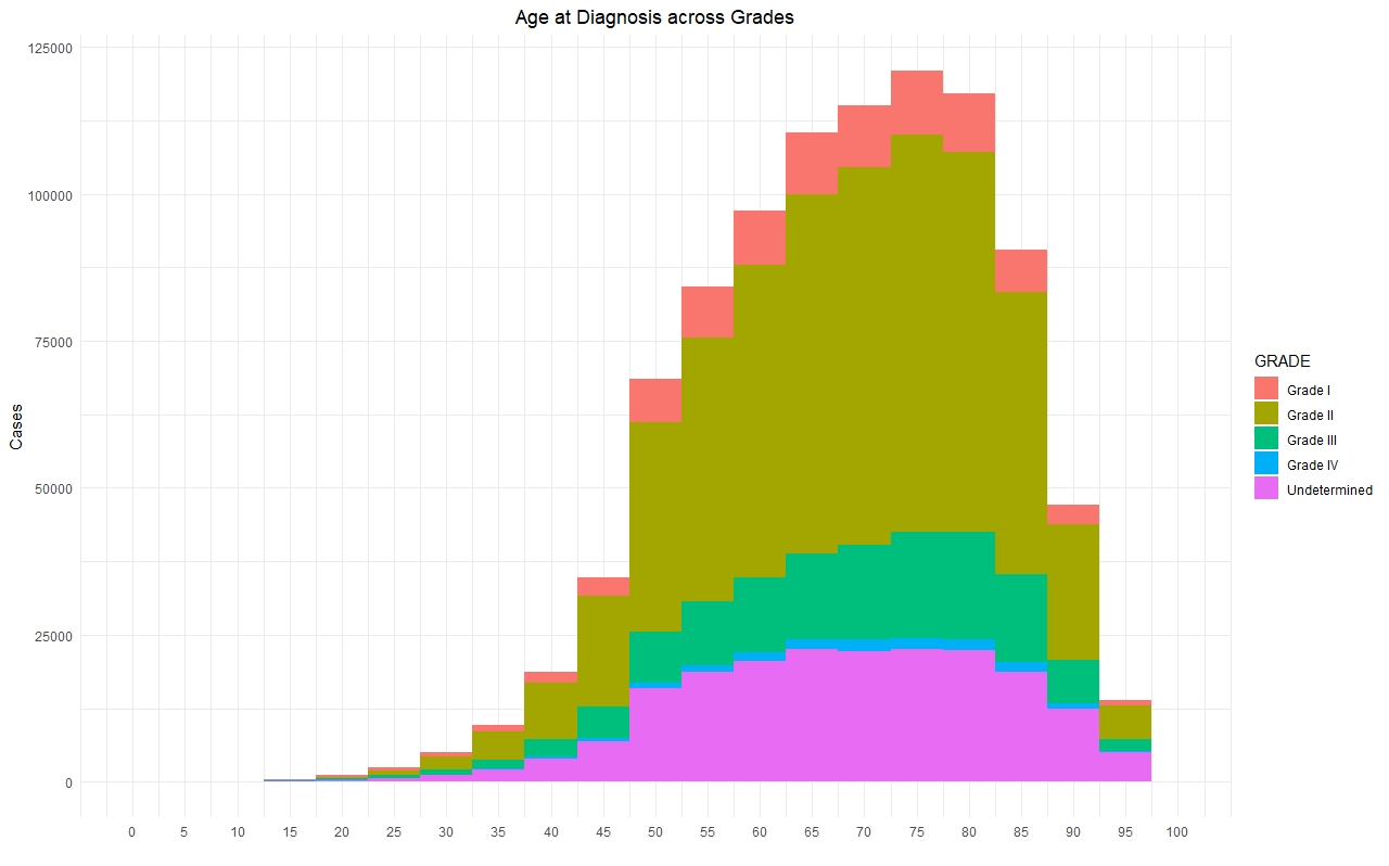
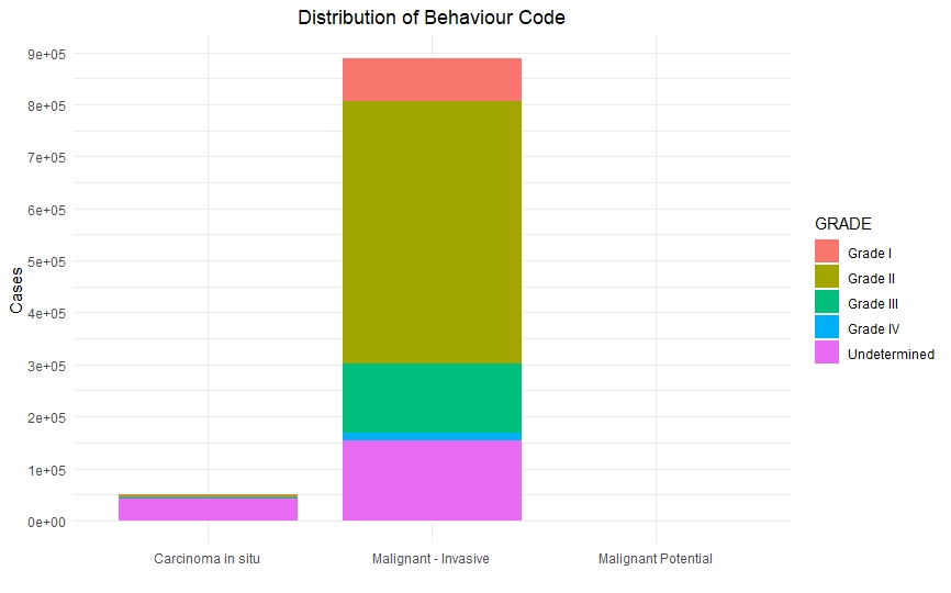
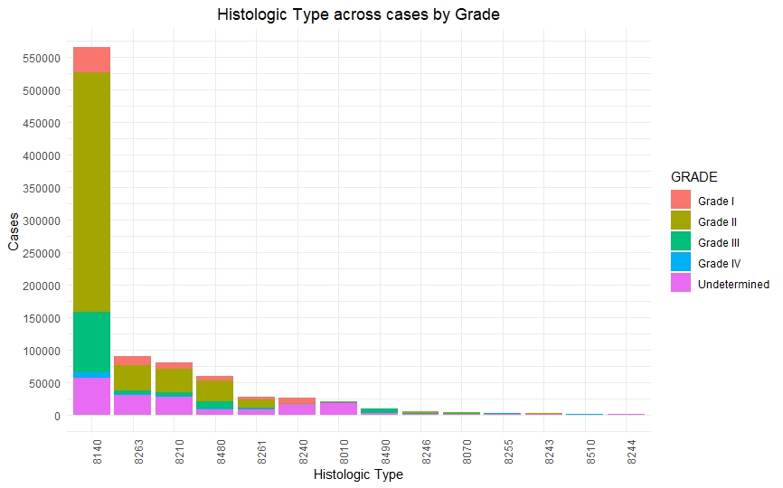
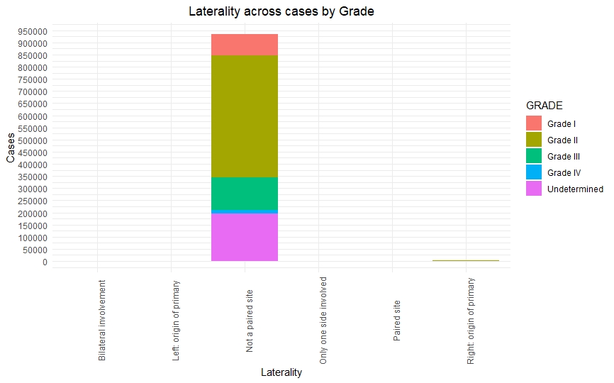
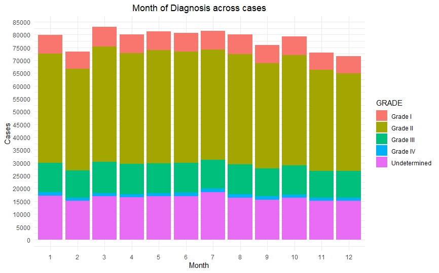
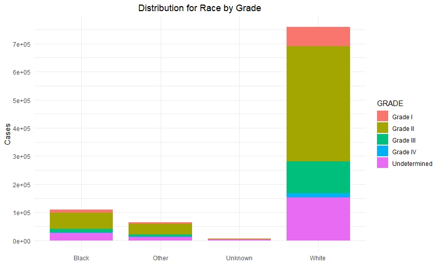
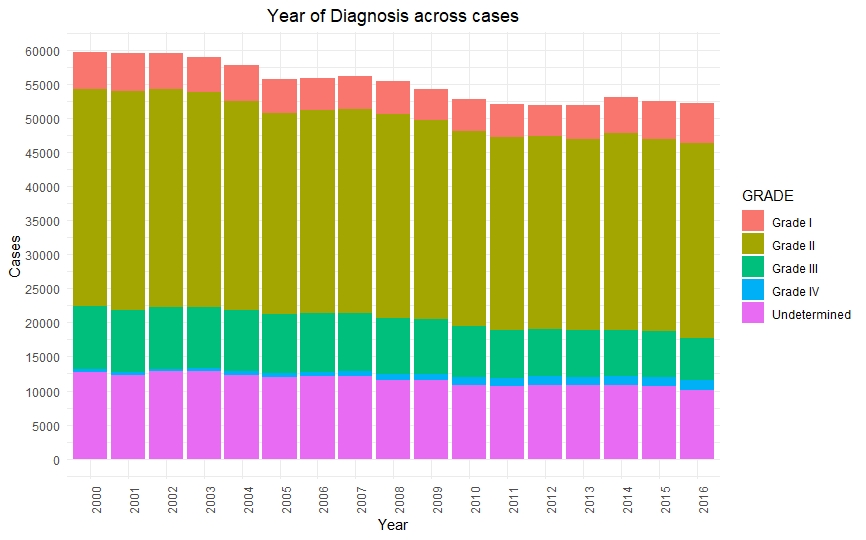
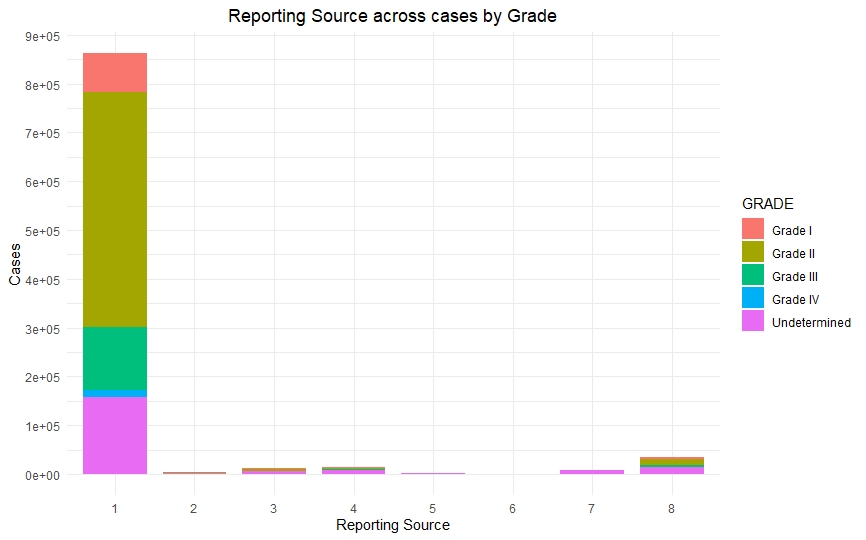
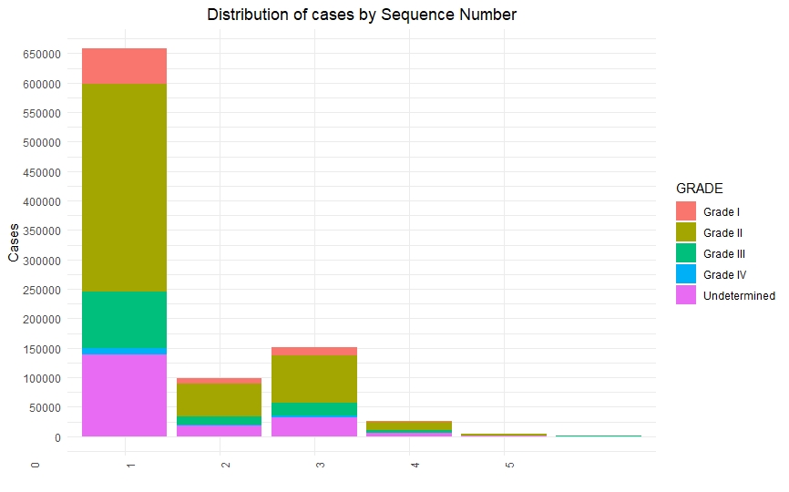
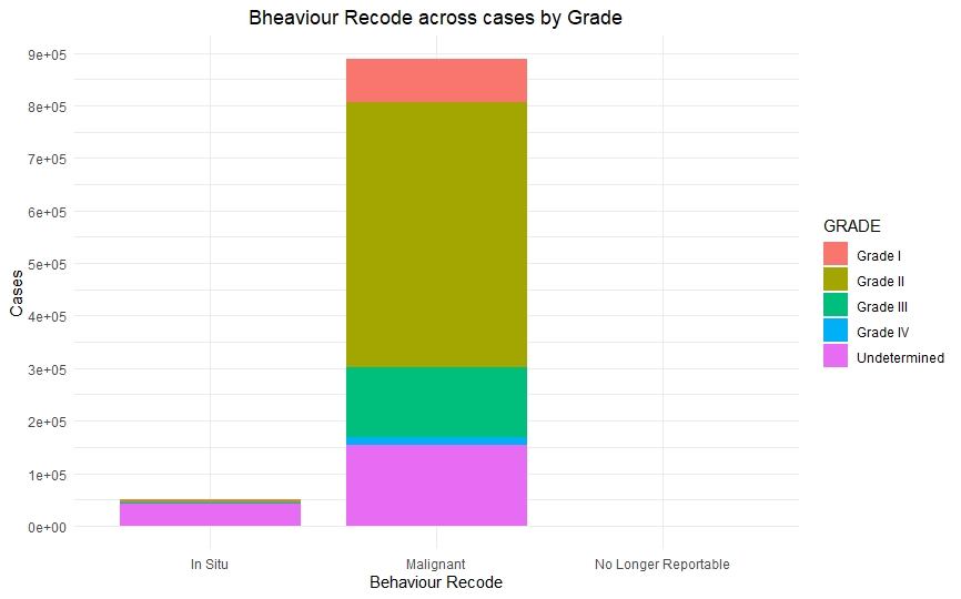
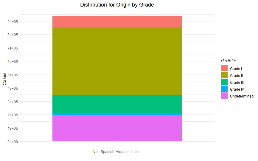
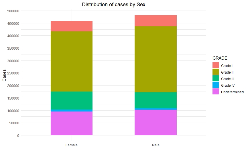
Data Visualization

Once we had a clean and consistent dataset, we created some visualizations to understand and represent the data we were working on. All of these plots are self-explanatory.

Predictive Models

We fit several predictive models. We started with simple models like Regression and Decision Trees. Though we got a good baseline with these models, we were hardly able to get some convincing results from these models.
Other models like Random Forest and Support Vector Machines hardly showed any increment in accuracy.
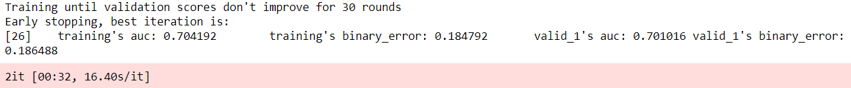
That’s when we decided to build some tree-based ensemble models. We then built models like XGBoost, LGBM (Light Grading Boosting Machine), and Catboost and kept improving them further until we got acceptable accuracy.

Model Validation

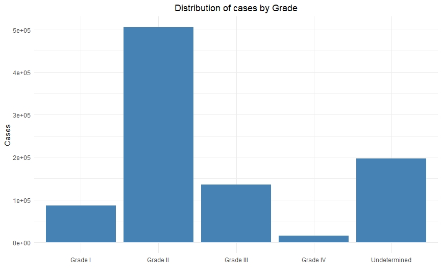
Real world projects like these is where making sure the models are statistically valid becomes the crucial step. Since the data is highly imbalanced (more people have grade I and grade II cancer than grade III and grade IV), the model too will be skewed towards the majority class. This is where approaches like cross-validation which show pessimistic bias, along with precision and recall, will give you most valid results.

Final Results

We were able to achieve an accuracy of ~80% with our LGBM models, which is still not good enough, but we managed to achieve an AUC (area under curve) of 0.71 which was on par with state-of-the-art AUV of average survivability prediction (0.79) source: https://www.researchgate.net/publication/318661649)

References

All statistics in this report are based on statistics from SEER and the Centers for Disease Control and Prevention’s National Center for Health Statistics. Most can be found within:

Howlader N, Noone AM, Krapcho M, Miller D, Brest A, Yu M, Ruhl J, Tatalovich Z, Mariotto A, Lewis DR, Chen HS, Feuer EJ, Cronin KA (eds). SEER Cancer Statistics Review, 1975-2016, National Cancer Institute. Bethesda, MD, https://seer.cancer.gov/csr/1975_2016/, based on November 2018 SEER data submission, posted to the SEER web site, April 2019.