Background

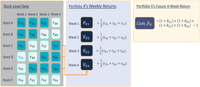
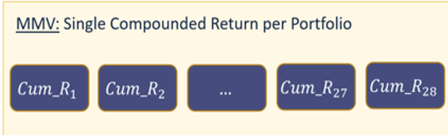
Factor portfolio is a portfolio of stocks where inclusion is defined by a single factor, such as book to price, 12-month return, and 12-month volatility. In this project, our objective was to develop a system that consumes stock-level signal data and recommends a factor policy (i.e. an allocation to each factor portfolio) which maximizes reward while controlling risk. We developed a pipeline system to combine inputs with models to generate weights and resulting performance metrics. We used Markowitz Mean-Variance and Principal Component Analysis (PCA) model to generate weights for factor portfolios.

Markowitz Mean-Variance Model (MMV)

Asset allocation is the strategy of dividing an investment portfolio across various asset classes like stocks and bonds. Essentially, asset allocation is an organized and effective method of diversification, which can help investors minimize risk while meeting an expected level of return. In this project, we are focused only on the stock market.\ Recently, researchers have been developing different methods for asset allocation. The Markowitz Mean Variance model is the most popular and widely-used one among them. It uses the statistical measure of expected return and variance to quantify the returns and the risk, respectively, of a security. It also considers the trade-off between return and risk in terms of a biobjective model: one objective is to minimize the variance of returns and the other is to maximize the expectation of returns. However, it is difficult to solve a bi-objective problem since in general, no single solution exists that simultaneously optimizes each objective. There are multiple ways to deal with this difficulty. For example, we can reformulate one objective function, either the objective of risk or the objective of return, as a constraint to set the maximum threshold for risk or minimum threshold for return. Another way is to linearly combine these two objectives. The third way is to take the advantage of the degree of concavity of the utility function to represent the investor’s attitude towards risk. If the utility function is concave, it means the investor is risk-averse. On the contrary, the convex utility function indicates that the investor is risk-seeking.

Principal Component Analysis

PCA decomposes the matrix of returns to analyze the variation in returns and gives loadings for each Principal Component (PC) which represent risk factors associated with portfolios. The loadings are used to generate asset weights towards each factor portfolio. Three approaches were reviewed and analyzed to generate asset weights from PC loadings and a method was proposed to select the best model parameter. The performance of both the models was analyzed using perfect information but the models were designed to work on estimated future data.

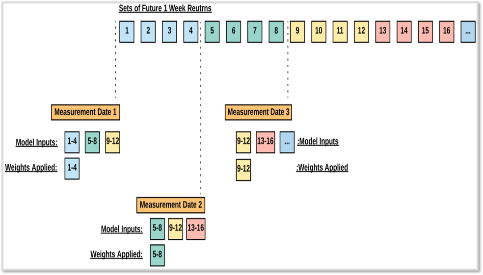
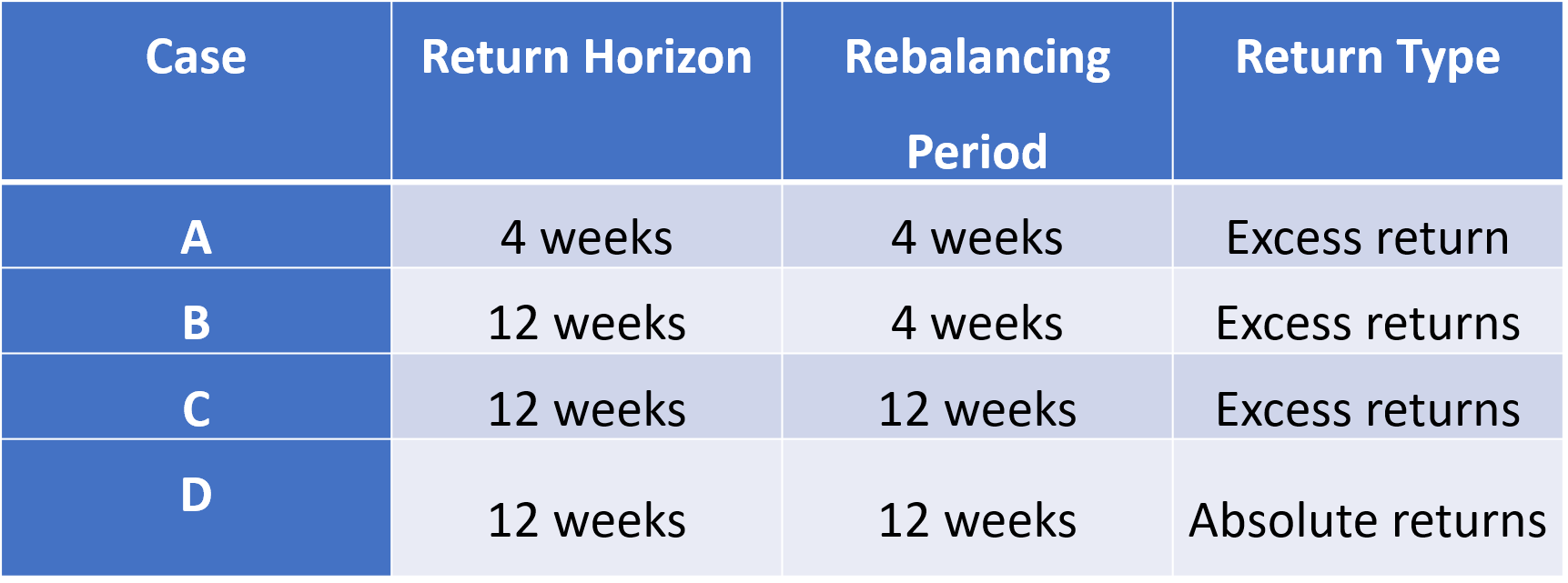
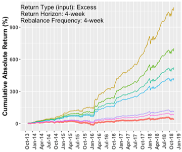
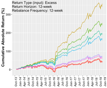
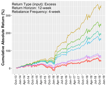
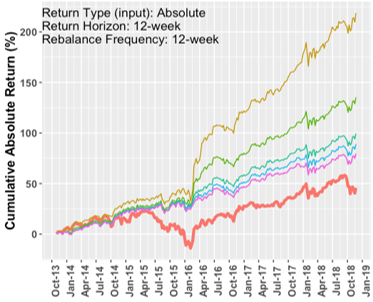
Differet Types of Input for Comparison

Sample evaluation process using a 12-week return horizon and a 4-week rebalancing period

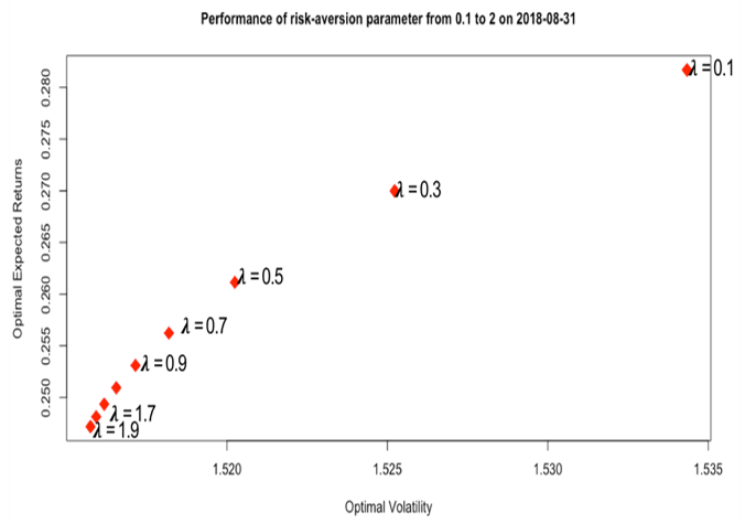
Comparisons for MMV model

When changing the risk-aversion parameter, we can see how it can affect the optimal volatility and expectation of portfolio returns by this efficient frontier plot.

Comparisons for PCA model

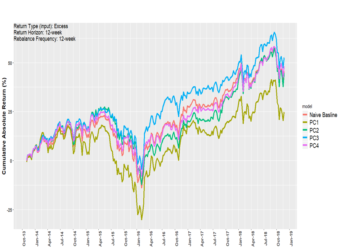
We can see that PCs describing most variation don’t necessary perform better than the Naïve-Baseline model.

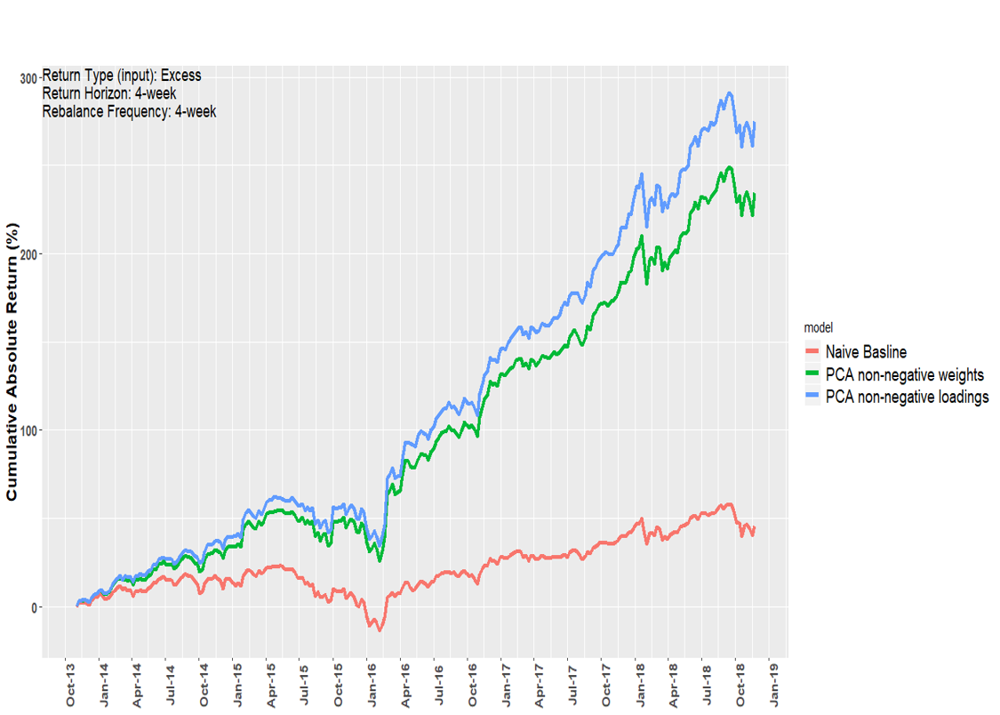Here, we can see that when we select best PC for each rebalancing period, the model outperforms the Naïve-Baseline model.

Cumulative Returns for best PC with different input parameters

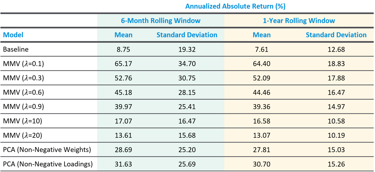
Comparison between MMV and PCA

Discussion and Recommendations

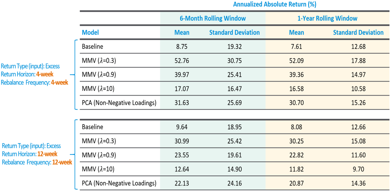
Our analysis examined how the Markowitz Mean-Variance, Principal Component Analysis, and Naïve Baseline models perform given perfect information about future returns. The MMV and PCA models show some similarities. Both are able to generate returns in excess of the baseline model. The standard deviation in annualized returns for MMV and PCA can be significantly higher than the baseline standard deviation under a 6-month window. But the standard deviation for both models decreases as we shift to a 1-year window. Both models favor the shorter 4-week return horizon and rebalancing periods. Both models favor the use of excess return inputs over absolute return inputs.\

But there are two important differences between the MMV and PCA models. First, we can find a specific value for the MMV risk-aversion parameter 𝜆 which will generate the same standard deviation in annualized returns as PCA but will generate high mean returns. We can find a MMV model to generate higher returns for the same risk. Second the MMV model provides a continuous range of possible 𝜆 risk aversion parameters which allow the investor to select from a combination of return and volatility combinations. For these reasons we recommend using the MMV model given perfect future information.\

While our analysis under perfect future information is an unrealistic scenario, we think this provides useful insight into how these models fundamentally work. Our analysis also provides a valuable benchmark against which Principal can compare results generated using estimated future returns. In addition to analyzing these models with imperfect information, we recommend that future work consider alternative measures of risk and use different time periods where the market exhibits different behaviors. Improvements to the models could include the addition of real-world investing constraints such as transaction costs or the requirement for a minimum level of diversification. The MMV model we analyzed assumed an investor’s risk-aversion parameter remained constant. The MMV model could be improved by making this parameter dynamic, reflecting true changes in risk tolerance that happen in different economic periods.\

We find that PCA is an interesting technique to study the market. We can use different approaches for PCA to study the variation in data and design our allocation strategy based on it. The final recommendation of parameters for PCA model would be using 4 week return horizon, 4 week rebalancing period, and excess returns.\

Using non-negative weights does give us higher results than the baseline, but it still cannot be said as the best model. Since, we don’t intend to short the stocks, the model currently has no strategy to deal with negative weights, other than eliminating it. We can research further to find a better strategy to deal with negative weights.