Ajinkya Koshti

Hi! My name is Ajinkya and I'm a data scientist located in Ames, IA.
I specialize in unstacking business value of data and delayering complex problems with state-of-the-art data science techniques. For more details, check out the About Me section.
View My LinkedIn Profile
The Idea
Earthquakes has devastating consequences in terms of living and financial cost. The GeoNet project locates 50 to 80 earthquakes each day and 20000 per year. Hence, forecasting the size and the timing of earthquakes becomes a significant challenge.[1] Los Almos National Laboratory (LANL) tries to solve this challenge by make available the seismic data obtained from laboratory earthquakes for data scientists to work upon. The data is labeled with the time it took for the lab sample to undergo an earthquake. We use this data to train a predictive model, fine-tune it and test on unseen data. We tested several machine learning algorithms to reduce the Mean Absolute Error (MAE) between actual and predicted times until next earthquake.
Background
This challenge is hosted on Kaggle by Los Alamos National Laboratory which enhances national security by ensuring the safety of the U.S. nuclear stockpile, developing technologies to reduce threats from weapons of mass destruction, and solving problems related to energy, environment, infrastructure, health, and global security concerns.
In this project, we show that by detecting the acoustic signal emitted by a laboratory fault, data science can predict the time remaining before it fails with great accuracy. These predictions are based solely on the instantaneous physical characteristics of the acoustical signal, and do not make use of its history. Surprisingly, machine learning identifies a signal emitted from the fault zone previously thought to be low-amplitude noise that enables failure forecasting throughout the laboratory quake cycle. We hypothesize that applying this approach to continuous seismic data may lead to significant advances in identifying currently unknown signals, in providing new insights into fault physics, and in placing bounds on fault failure times. [2]
Data Description
The data comes from a well-known experimental set-up used to study earthquake physics. The “acoustic_data” input signal is used to predict the time remaining before the next laboratory earthquake (time_to_failure).
The training data is a single, continuous segment of experimental data. The test data consists of a folder containing many small segments. The data within each test file is continuous, but the test files do not represent a continuous segment of the experiment; thus, the predictions cannot be assumed to follow the same regular pattern seen in the training file.
For each “seg_id” in the test folder, you should predict a single “time_to_failure” corresponding to the time between the last row of the segment and the next laboratory earthquake.
Data Fields
- acoustic_data - the seismic signal [int16]
- time_to_failure - the time (in seconds) until the next laboratory earthquake [float64]
- seg_id - the test segment ids for which predictions should be made (one prediction per segment)
Data Exploration
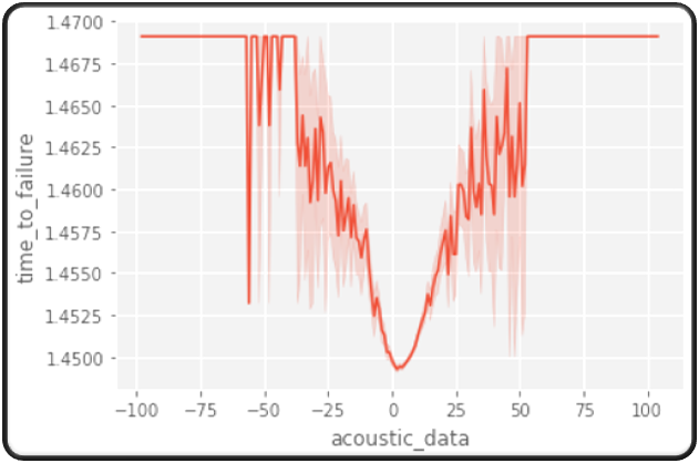
Since, we only have one feature, there isn’t much to visualize. The only inference we can make from this plot is the time-series of the acoustic data.
Feature Engineering
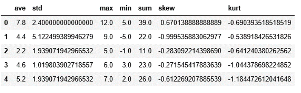
Our dataset has 629 million datapoints but only one attribute. So, it was quite impossible for the models to learn the patterns in data with just one attribute. Hence, to overcome this problem we implemented feature engineering. Feature engineering is the process of using domain knowledge of the data to create features that make machine learning algorithms learn better. We constrict intermediate features from the original descriptors in a dataset. Since, we only have one attribute, we aggregate a few datapoints together and calculate the statistical features as mean, standard deviation, skew, kurtosis, etc. These statistical features give us a holistic overview of the segment of the data, which then helps our algorithms learn better.
Denoised Features
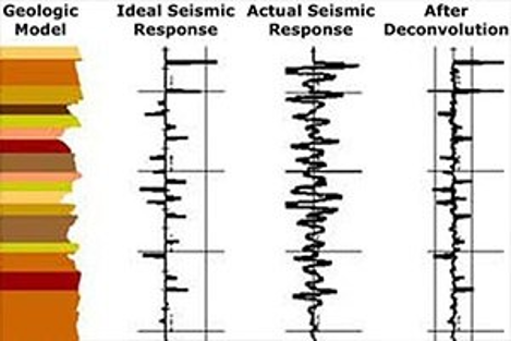
In previous task, we just created statistical aggregations of the data segments. Though, it helped our algorithm learn better and consequently, increase our accuracy, we learned that there still were better approaches. We found an article on kaggle explaining the seismologic process of measuring seismic signals and found out the limitations in that process. The limitation was that the original seismic signals are quite difficult to record and measure, hence an artificial signal is used to amplify the actual signal. Thus, the recorded signal is always a mixture of actual + artificial amplified signal. Thus, to use the actual signal for our analysis, which arguably might give us better results, we need to denoise this signal. Since, these denoising calculations require high domain expertise, for the sake of this project we decided to follow the procedures in Kaggle notebook [3], which is an open-source data science platform. The constructed denoised features then represented the actual signal.
Data Pre-processing
Data preprocessing is a data mining technique that involves transforming raw data into an understandable format. Real-world data is often incomplete, inconsistent, and/or lacking in certain behaviors or trends, and is likely to contain many errors. Data preprocessing is a proven method of resolving such issues.
Fortunately, we had a well-curated and consistent data with only attribute, so there was no pre-processing required. The only pre-processing, we did was to segment and sample the data to test our algorithms, and to connect kaggle/google drive APIs with google colab for our analysis. Since the data file was of 9GB we had to spend good amount of time in appropriately sampling it and in saving it as a pickle file, which is a format that saves files in much smaller size than its original size.
Correlation Analysis
Correlation analysis is a statistical method used to evaluate the strength of relationship between two quantitative variables. A high correlation means that two or more variables have a strong relationship with each other, while a weak correlation means that the variables are hardly related. In other words, it is the process of studying the strength of that relationship with available statistical data.
Multicollinearity increases the standard errors of the coefficients. Increased standard errors in turn means that coefficients for some independent variables may be found not to be significantly different from 0. In other words, by overinflating the standard errors, multicollinearity makes some variables statistically insignificant when they should be significant. Without multicollinearity (and thus, with lower standard errors), those coefficients might be significant.
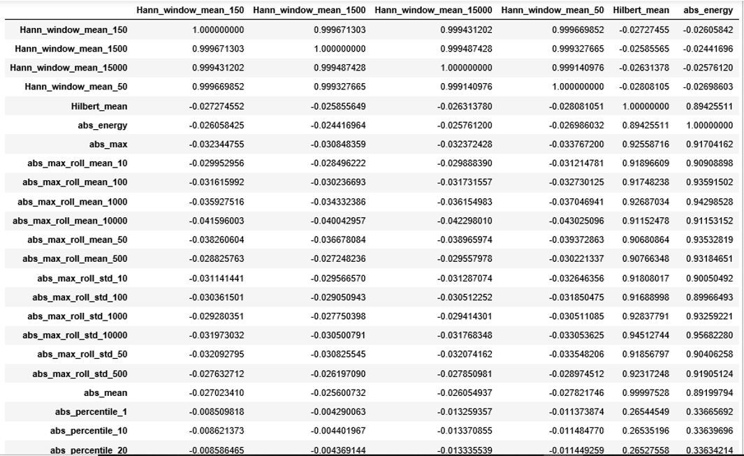
In the denoised the data set we had 979 attributes which are statistically generated. As these features are generated statistically in correlation matrix some of the attributes were highly correlated to each other. So, we set a cut-off value of .95 and removed highly corelated data points from the denoised data. After correlation we had 644 attributes.
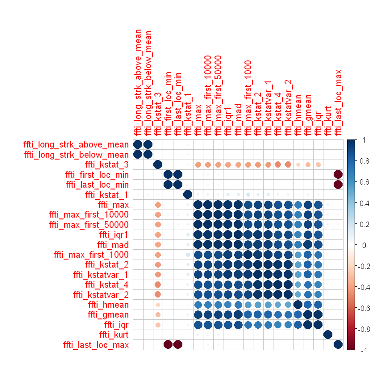
Note: Correlation plot is difficult to visualize with as many features as we have. Hence, we directly exported them in excel and used a code to set the threshold to elimiate highly correlated features. The above snapshot is just to give an idea of how highly correlated the similar statistical features can be.
Predictive Models
We modeled the given data on several predictive models such as Random Forest, Support Vector Machine and some gradient boosted models such as Light Gradient Boosting Machine, Catboost and XGboost.
Random forest train each tree independently, using a random sample of the data. This randomness helps to make the model more robust than a single decision tree, and less likely to overfit on the training data. The RF model is an average over a set of decision trees. Each decision tree predicts the time remaining before the next failure using a sequence of decisions based on statistical features derived from the time windows.
Gradient boosted trees build trees one at a time, where each new tree helps to correct errors made by previously trained tree. GBM and RF differ in the way the trees are built: the order and the way the results are combined. GBM performs better than RF if parameters are tuned carefully.
LGBM (Light Gradient Boosting Machines)
Light GBM is a gradient boosting framework that uses tree-based learning algorithm. Light GBM grows tree vertically while other algorithms grow trees horizontally which means that Light GBM grows tree leaf-wise while other algorithms grow level-wise. It will choose the leaf with max delta loss to grow. When growing the same leaf, Leaf-wise algorithm can reduce more loss than a level-wise algorithm [4].
XGBoost
XGBoost fits a model on the gradient of loss generated from the previous step. In XGBoost, just gradient boosting algorithm is modified so that it works with any differentiable loss function [5]. Gradient boosting is an approach where new models are created that predict the residuals or errors of prior models and then added together to make the final prediction. It is called gradient boosting because it uses a gradient descent algorithm to minimize the loss when adding new models.
Catboost
CatBoost is based on gradient boosting. A new machine learning technique developed by Yandex that outperforms many existing boosting algorithms like XGBoost, Light GBM. One main difference between CatBoost and other boosting algorithms is that the CatBoost implements symmetric trees. This helps in decreasing prediction time, which is extremely important for low latency environments. CatBoost does gradient boosting in an ordered boosting manner. Ordered boosting can be computetionally expensive if we train the data for each data point. So, instead catboost trains the mfel for log(number of datapoints)[6].
Results
Statistical aggregations as features
| Predictive Models | MAE (in seconds) |
|---|---|
| Random Forest | 2.389 |
| SVM | 2.286 |
| LGBM | 2.23 |
| Catboost | 1.33 |
Denoised features
| Predictive Models | MAE (in seconds) |
|---|---|
| Random Forest | 1.26 |
| SVM | 2.092 |
| LGBM | 1.323 |
| Catboost | 0.87 |
| XGBoost | 0.89 |
Conclusion
- It is possible to predict time until earthquake from seismic vibrations.
- If we can successfully scale this model and translate the results from lab samples to the actual ground sites, then it can help decision-makers potentially save billions in disaster mitigation activities.
- Advanced gradient based tree models have potential to learn from and identify patterns in big data.
- Computation time becomes a big issue as the size of data increases. It then becomes an important challenge to achieve a tradeoff between computation time and prediction accuracy.
- Statistical aggregations can help create new features for more accurate analysis.
References
- Machine Learning Can Predict the Timing and Size of Analog Earthquakes (F. Corbi,L Sandri, J. Bedford , F. Funiciello, S. Brizzi, M. Rosenau, S. Lallemand, 2019)
- Machine Learning Predicts Laboratory Earthquakes (Bertrand Rouet‐Leduc, Claudia Hulbert, Nicholas Lubbers, Kipton Barros, Colin J. Humphreys, Paul A. Johnson, 2017)
- https://www.kaggle.com/tarunpaparaju/lanl-earthquake-prediction-signal-denoising
- https://medium.com/@pushkarmandot/https-medium-com-pushkarmandot-what-is-lightgbm-how-to-implement-it-how-to-fine-tune-the-parameters-60347819b7fc
- https://medium.com/@pushkarmandot/how-exactly-xgboost-works-a320d9b8aeef
- https://medium.com/@hanishsidhu/whats-so-special-about-catboost-335d64d754ae